Lab 7: Phonation Types
Thomas Kettig, based on work by Sonya Bird et al.
Goal of Lab 7:
In this lab we are going to explore the acoustic correlates of the three main phonation types used across languages: modal voicing, creaky voicing, and breathy voicing. This lab deals with a large number of measurements, so I would encourage working together in pairs for this report!
SOUND FILES
Go to eClass and download the sound files:
| File name |
|---|
| Lab7_breathyvoice.wav |
| Lab7_modalvoice.wav |
| Lab7_creakyvoice.wav |
Once these files have been downloaded, open them in Praat and fill in the cells of Table 7.1 on the lab report to compare voicing types in terms of different parameters. The table will be very large, so you may want to split it up over a few pages in such a way that each time you start a new page, the table header is repeated (otherwise, it won’t be possible for your reader to know what column goes with what measurement!). Follow the instructions below for taking the appropriate measurements.
INSTRUCTIONS
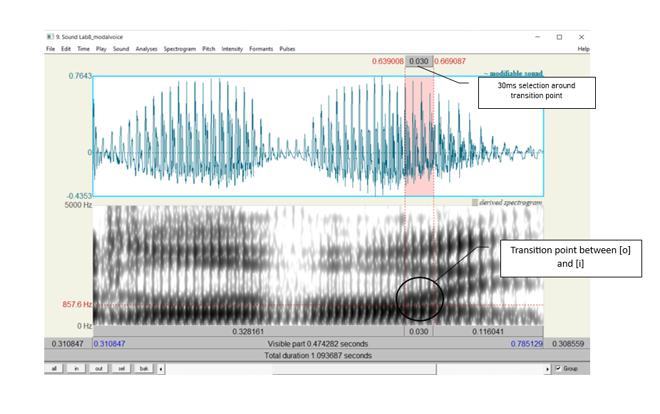
Since the word “voice” occurs in all three recordings, this is a good word to use for comparing across phonation types. Unless otherwise noted, measurements should be taken around the transition point between [o] and [i] in [oi] of voice, i.e. where the formants start spreading out. Each measurement may require a different length of speech to get the best results, so approximate durations to measure are provided in the instructions for each. Here are approximate transition points in each file around which you can centre your measurements:
- Modal voicing: 0.640s (see Figure 7.1)
- Creaky voicing: 0.703s
- Breathy voicing: 0.654s
TIP: Keep in mind that what matters in comparing measurements are relative values rather than absolute values. For example, in analyzing jitter, what matters is which phonation type has the most jitter, not what the exact measurement is.
A. FUNDAMENTAL FREQUENCY (F0)
Fundamental frequency can be a good indication of phonation type. Note down F0 averaged over about 30ms around the transition point of [oi] for the three phonation types in Table 7.1 (if you can’t remember how to do this, see Lab 3).
TIP:
When you select a range in the view window, the values of F0 and amplitude at the right of the view window will report averages calculated over the selected region. Note, however that this does not work for formants (displayed at the left) because there are usually many formants at any point in time, but just one average F0/amplitutde.
B. PERIODICITY
There are two things to consider here:
- How regularly the pitch pulses occur = degree of periodicity in the waveform
- How many higher-frequency components there are in the waveform = spectral noise
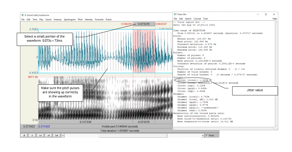
The degree of periodicity can be quantified by measuring the jitter: the variation in the duration of successive F0 cycles (see Figure 7.2). Follow the instructions below and note down your jitter measurements.
TIP:
You will not be able to get a jitter value unless the pitch pulses are showing up correctly in the waveform (the vertical lines on the waveform, see Figure 7.2). If at the suggested point of measurement in transition of [oi] there are no pitch pulses, measure jitter at some other point where you do see the pitch pulses.If you notice that there are no pitch pulses on the waveform, you might need to adjust the ‘Pitch’ settings! Go to Pitch and click the “Standards’ button. This will reset any previous settings and might help show the pitch pulses on the waveform.
- Measure jitter value:
- Pulses > Show pulses.
- Select a portion of the waveform around the centre of the /oi/ vowel (OR where you see pitch pulses clearly) which is around 70-80ms.
- Pulses > Voice report.
- In the report window, find the value for Jitter (local), and note this down in Table 7.1.
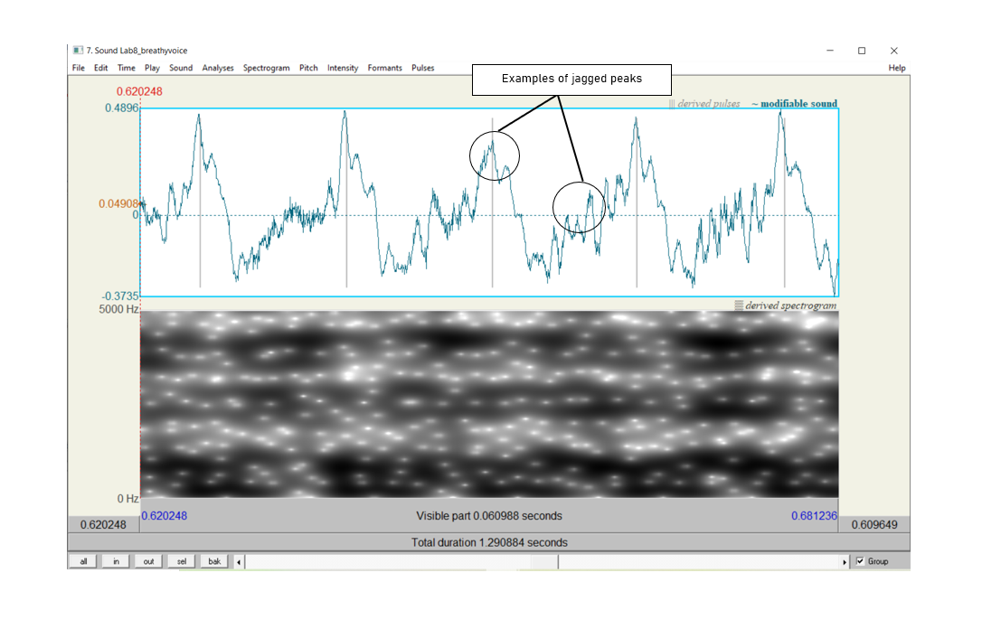
On the waveform you can also see how much spectral noise there is in the signal by how complex the waveform looks (see Figure 7.3).
Zoom in on the waveform until you can clearly see a few cycles (Figure 7.3). Note down in Table 7.1 your judgment on how much noise you observe.
C. ACOUSTIC INTENSITY
The three phonation types also differ in intensity. There are two ways to think about intensity differences, introduced below.
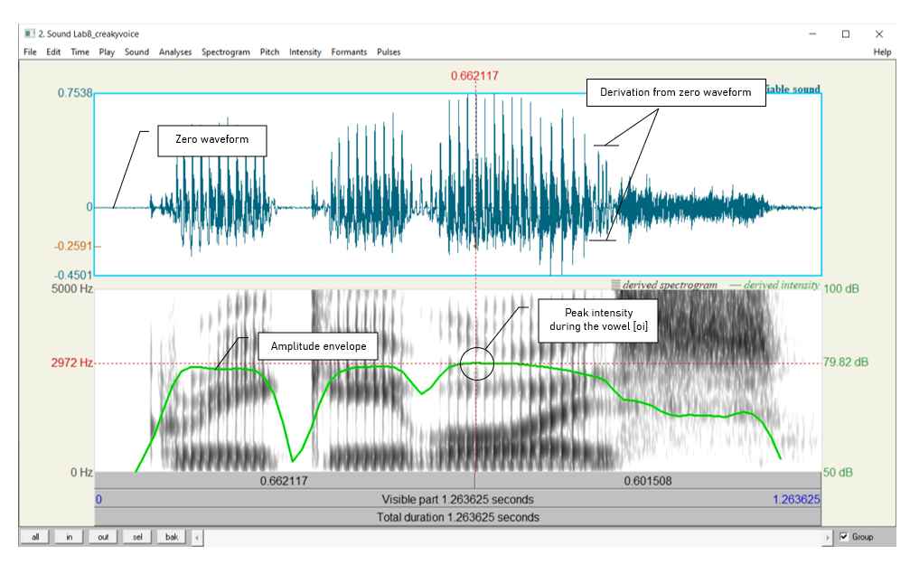
- Acoustic intensity can be ‘eyeballed’ by viewing the waveform or spectrogram directly. Note down the relative darkness on spectrogram and the relative size of deviations from zero waveform for different phonation types in Table 7.1.
Amplitude can also be quantified by viewing the amplitude envelope (green contour) on the spectrogram display (see Figure 7.4). Note down in Table 7.1 the green amplitude value (in dB) on the right of the screen for different phonation types.
- Intensity > Show intensity
- Find the peak intensity (the highest point on green amplitude contour) during the vowel [oi]
- Click on the amplitude contour at this point
- Note the green amplitude value (in dB) on the right of the screen
D. SPECTRAL TILT
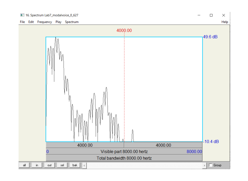
Spectral tilt is the degree to which intensity drops off as frequency increases. It can be eyeballed by looking at a spectral slice of the waveform, which gives the component frequencies and their amplitudes (see Figure 7.5). Note down the overall slope of the spectrum for different phonation types in Table 7.1 (steep, gradual, etc.).
- Select about 50-60ms of the waveform around the measurement point given above.
- Spectrum > View spectral slice
- The overall slope of the spectrum (= how quickly the amplitude drops off in the higher frequencies, above the F1 peak) is an indication of spectral tilt.
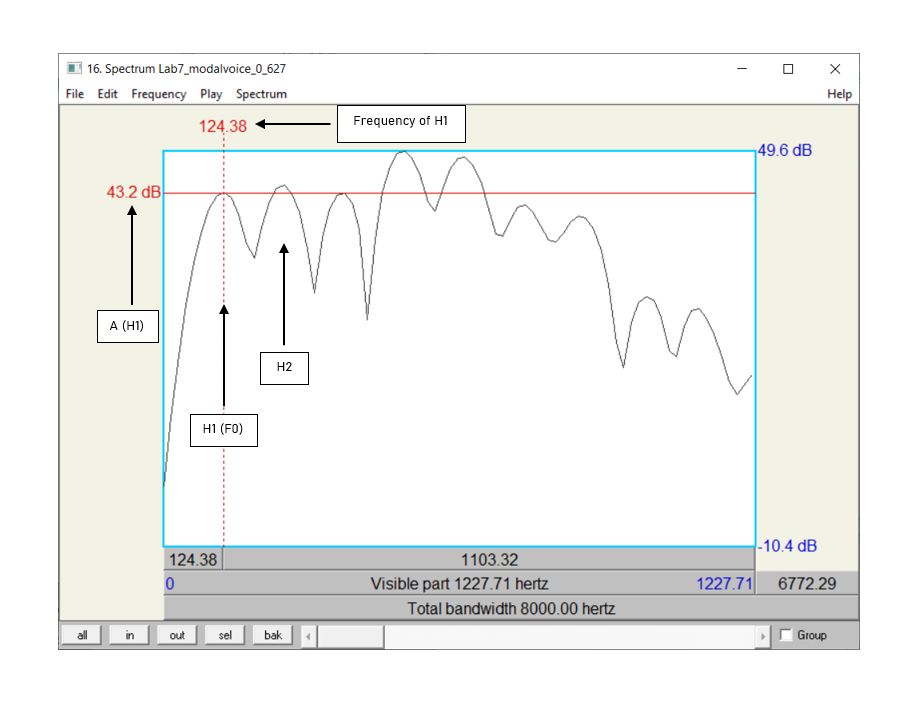
Spectral tilt can be quantified by comparing the amplitude of F0 to that of higher frequency harmonics, e.g. the second harmonic, the harmonic closest to the first formant, or the harmonic closest to the second formant. The easiest way to measure spectral tilt is by subtracting the amplitude of the second harmonic (H2) from the amplitude of F0 (H1) (see Figure 7.6). Fill in Table 7.1 with the spectral tilt value of the three phonation types.
- In the spectral slice, select the first ~10 peaks (that is, the first ~10 harmonics) and zoom in so that you can see H1 and H2 clearly.
- Click on the peak of H1 and get its amplitude - the number on the left of the screen corresponds to the amplitude; the number at the top of the screen corresponds to the frequency.
- Click on the peak of H2 and get its amplitude.
- Calculate spectral tilt by this formula: A(H1)-A(H2), that is, the amplitude of H1 minus the amplitude of H2. (No need to worry about frequencies for this measure, only amplitudes.)
TIP:
H1 is the first big-sized peak; H2 is the second one. There may be one or two lower amplitude peaks before H1, so make sure you’re measuring the right peaks. If you click on the first big peak (H1), the value at the top of the vertical red bar gives you its frequency. Make sure this frequency corresponds to F0 (as verified by some other measurement technique – see Lab 3). Also make sure that the frequency of H2 is approximately twice the frequency of H1 (see Lab 4 for the reasoning here).
E. FORMANT FREQUENCY
Non-modal phonation can affect the formant frequencies, particularly the first formant (F1). Note down F1 for each phonation type.
- For this measurement, select about 30ms in the stable (middle) part of the [o] portion of the [oi] diphthong, not the transition point between [o] and [i].
- On the spectrogram, click in the centre (vertical) of the first formant (F1).
- The number at the left of the screen at the end of the red horizontal bar gives you the frequency (in Hz).
TIP:
You can use the formant tracings if they help: Formant > Show formants.
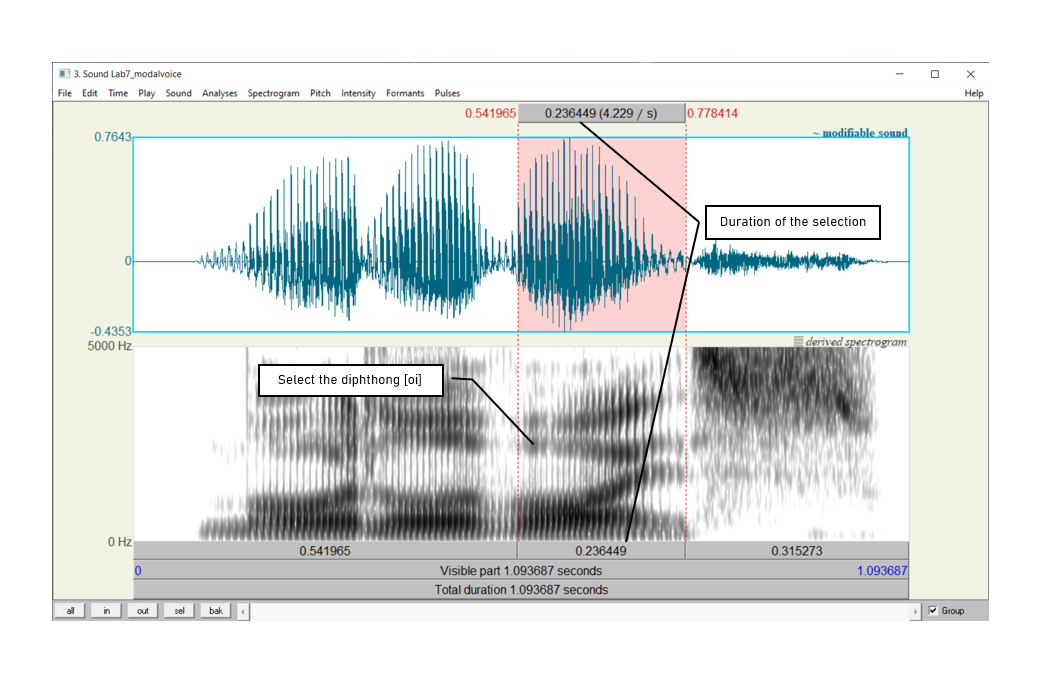
F. DURATION OF [oi]
Duration can also be an indication of phonation type (see Figure 7.7). Note down the duration of [oi] for each phonation type.
- Measure the duration for the whole diphthong [oi] by selecting the vowel
- You can read the duration from the panel above the selected segment
TIP:
To isolate [oi], you can use visual information (look for the change in the shape of the spectrogram/waveform). You can also use your ears to verify that you haven’t captured any portions of the preceding [v] or following [s].
G. OVERALL CLARITY OF THE SPECTROGRAM
Finally, phonation types differ in the overall clarity of the spectrogram, which mainly has to do with the amount of noise in the signal. Note down your impressions of overall clarity of the spectrogram of each phonation type - e.g. how clear or blurry are the formants?
LAB 7 REPORT
Table 7.1 Comparing acoustic correlates of different phonation types (enter values where measurements were taken; otherwise enter general comments)
| Modal voicing | Creaky voicing | Breathy voicing | ||
|---|---|---|---|---|
| 1. Fundamental frequency | ||||
| Periodicity | 2. Jitter value | |||
| 3. Spectral noise | ||||
| Intensity | 4. Relative darkness on spectrogram / relative deviation on waveform | |||
| 5. Amplitude value (dB) | ||||
| Spectral tilt | 6. Overall slope of the spectrum | |||
| 7. A(H1) - A(H2) | ||||
| 8. Formant frequency (F1 value) | ||||
| 9. Duration of [oi] (ms) | ||||
| 10. Overall clarity of spectrogram |
Q1: Based on your observations, what measurements/cues seem to be the most and least reliable for distinguishing phonation types, at least with this speaker’s voice?
REFERENCES
Q2: Provide a reference and very brief summary of one academic paper that uses the methods covered in this lab.
Disclaimer: The original lab materials on which this lab is based was put together in 2015 (updated 2019) by Sonya Bird, Qian Wang, Sky Onosson, and Allison Benner for the LING 380 Acoustic Phonetics course at the University of Victoria. Their materials are released under a Creative Commons license (CC BY-NC-SA 4.0) which allows for non-commercial use as well as copying and distribution and the creation of derivative works for non-commercial purposes. Thomas Kettig (with assistance from Taylor Potter) has modified these materials as needed for the York University LING 4220 Acoustic Phonetics course.